 LINGCORE SCI
Flexible Parametric Survival Models: Royston–Parmar
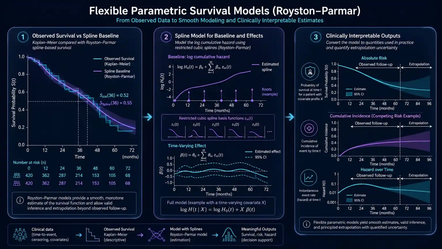
Flexible parametric survival models, especially the Royston–Parmar model, use restricted cubic splines to model the baseline survival process smoothly. They can produce absolute survival and risk estimates at arbitrary time points, represent time-varying effects, and support competing-risk or extrapolation analyses, but their credibility depends on knot choice, scale selection, validation, and transparent assumptions beyond observed follow-up.
Why move beyond a Cox baseline hazard?
The Cox proportional hazards model is valuable because it estimates relative effects without specifying the baseline hazard. That convenience also limits some clinical outputs. A standard Cox analysis does not directly parameterize a smooth baseline survival function, and absolute risk estimates are often obtained afterward through stepwise estimators at observed event times.
Flexible parametric survival models take a different route. They model a transformed baseline survival quantity with a parametric function, commonly a restricted cubic spline of log time. The resulting curve is smooth over the modeled time range. Researchers can estimate survival probability, cumulative hazard, hazard, risk differences, restricted mean survival time, and other quantities directly from the fitted model.
The gain is not that splines are automatically more correct. The gain is that the model makes the time structure explicit and allows clinical questions to be expressed on an absolute-risk scale. The cost is a greater need to justify the transformation, degrees of freedom, knot placement, effect scale, and behavior beyond the data.
What the Royston–Parmar model represents
In the proportional-hazards formulation, the model represents the log cumulative hazard as a smooth function of log time plus covariate effects:
The function s is a restricted cubic spline. It is constructed from basis functions joined at knots, with linear behavior in the tails beyond the boundary knots. The spline can represent a baseline cumulative hazard that changes direction over time, unlike a simple Weibull model whose hazard shape is constrained by a small number of parameters.
The same family can be fitted on other scales. A proportional-odds formulation models a transformation related to survival odds, and a probit or normal-scale formulation provides another link between the linear predictor and the survival function. The selected scale is part of the model specification, not a cosmetic choice.
Flexible parametric survival models versus common alternatives
| Model | Baseline time structure | Typical output | Key limitation |
|---|---|---|---|
| Cox proportional hazards | Unspecified baseline hazard | Hazard ratios; post-estimation survival curves | Proportional-hazards assumption; smooth absolute-risk modeling is not built into the primary likelihood |
| Weibull survival model | Parametric monotone hazard shape | Survival, hazard, and absolute risk | May be too restrictive when hazards are non-monotone or have multiple phases |
| Royston–Parmar model | Restricted cubic spline for a transformed baseline function | Continuous survival, hazard, risk, RMST, and time-varying effects | Knot choice, scale, overfitting, and extrapolation require explicit assessment |
| Piecewise exponential model | Constant hazard within prespecified intervals | Hazard and survival estimates by interval | Results depend on cut points; many intervals can create instability |
| Accelerated failure-time model | Distributional time-scale assumption | Time ratios and survival distributions | Interpretation and fit depend on the chosen distribution and acceleration structure |
Knot placement and degrees of freedom
The number of interior knots controls how much the baseline function can bend. Too few degrees of freedom may underfit important hazard changes. Too many can follow random fluctuations, especially when the number of events is limited. Knot placement also matters because the data may contain dense event information in one time region and sparse information in another.
Clinical researchers should report the number of knots, the scale on which the spline was fitted, the rule used to place knots, boundary handling, and any sensitivity analyses. A model is not reproducible when the article says only “a flexible parametric model was fitted.” The spline basis and time origin are part of the estimand’s operational definition.
Visual inspection should be paired with quantitative checks. Compare observed Kaplan–Meier or cumulative-incidence estimates with model-based curves, inspect calibration at clinically relevant horizons, examine residual or pseudo-residual behavior when available, and assess whether the fitted hazard has implausible oscillations. Knot selection should not be based solely on the lowest in-sample information criterion.
Time-varying effects within the model
A major advantage of flexible parametric survival models is that covariate effects can vary smoothly with time. Instead of imposing a constant coefficient β, the model can include an interaction between a covariate and spline functions of log time:
This allows a treatment effect or prognostic association to change over follow-up. The resulting curve may show an early treatment difference that attenuates, a delayed separation, or a changing association in chronic disease. Such patterns should be interpreted on the scale of the model and translated into time-specific hazard ratios, survival differences, risk differences, or RMST contrasts.
A time-varying coefficient is not evidence that the treatment effect truly changes biologically. It may reflect treatment switching, informative follow-up, competing events, non-proportional measurement processes, model misspecification, or random variation. The analysis should prespecify how time variation will be evaluated and should show uncertainty bands around the estimated effect.
Absolute risk and clinically interpretable estimands
Hazard ratios are relative measures. Clinical decisions often require absolute quantities: the probability of surviving to 12 months, the risk difference by 24 months, the number of events prevented per 1,000 patients, or the mean event-free time over a restricted horizon. Flexible parametric models are useful because they provide a smooth estimated survival function from which these quantities can be calculated at arbitrary times within the supported range.
For example, a treatment comparison can be expressed as survival probability under each treatment at 6, 12, and 24 months, an absolute risk difference at each horizon, or a restricted mean survival-time difference through 24 months. These summaries can be more interpretable than a single hazard ratio when hazards are non-proportional or when the clinical decision concerns a fixed time point.
Absolute predictions must be validated. A smooth curve can look persuasive while being miscalibrated. Report calibration-in-the-large, calibration slope or flexible calibration plots, prediction error, and uncertainty at prespecified horizons. If the model is intended for individual risk prediction, also assess transportability across sites, calendar periods, disease severity, and clinically important subgroups.
Competing risks and multiple event processes
When a competing event prevents the event of interest from occurring, standard survival probabilities require careful interpretation. Flexible parametric frameworks can be extended to model cause-specific hazards, cumulative incidence functions, or other competing-risk estimands. These are not interchangeable.
A cause-specific hazard describes the instantaneous event rate among individuals who are still free of any event. A cumulative incidence function describes the probability of experiencing a particular event by a time point in the presence of competing events. A model that produces a smooth cause-specific hazard does not automatically provide a direct model of the clinical probability of the event of interest. The article should name the estimand before describing the model.
For competing-risk analyses, report how event types were coded, whether covariates were allowed to have cause-specific time-varying effects, how cumulative incidence was derived, and how uncertainty was calculated. If the clinical question concerns treatment policy or resource planning, cumulative incidence and absolute risk may be more relevant than a cause-specific hazard ratio.
Extrapolation beyond observed follow-up
Flexible parametric models are frequently used to estimate survival beyond the end of a trial or registry. The smooth mathematical form makes extrapolation possible, but it does not make the extrapolated tail identifiable from the observed data. Once the curve extends beyond the region with reliable follow-up, the result is driven increasingly by the chosen functional form and external assumptions.
A defensible extrapolation analysis should show the observed follow-up boundary, identify where censoring becomes substantial, compare multiple plausible models, and perform sensitivity analyses using alternative tail behaviors. External mortality or registry information may help in relative-survival or health-economic settings, but such information must be aligned with population, calendar period, age, and outcome definitions.
Do not present a single extrapolated mean survival time as if it were observed. Display prediction intervals or confidence intervals, distinguish parameter uncertainty from structural uncertainty, and state which parts of the result depend on assumptions that cannot be checked using the trial data alone.
Five-step flexible survival modeling workflow
| Step | Action | Reporting output |
|---|---|---|
| Step 1: Define the estimand | Specify the event, competing events, time origin, follow-up, target population, scale, and whether the primary target is hazard, survival, risk, RMST, or cumulative incidence. | Versioned estimand and event-coding plan |
| Step 2: Diagnose the time structure | Inspect Kaplan–Meier or cumulative-incidence curves, event density, censoring, and plausible non-proportionality before choosing the baseline form. | Pre-model diagnostic plots and rationale |
| Step 3: Fit and compare candidate forms | Vary degrees of freedom, knot placement, link scale, and time-varying-effect terms; compare fit while prioritizing clinical plausibility. | Model specification and sensitivity table |
| Step 4: Validate absolute predictions | Assess calibration, discrimination, prediction error, subgroup performance, and uncertainty at prespecified horizons. | Validation plots and horizon-specific estimates |
| Step 5: Translate and stress-test | Report absolute risks, survival differences, RMST, or cumulative incidence; mark extrapolation and test alternative assumptions. | Clinically interpretable estimates with structural uncertainty |
Evidence Summary Table
| Source | Evidence type | Methodological contribution | Reporting implication |
|---|---|---|---|
| Royston and Parmar, Statistics in Medicine | Original methods paper | Introduced flexible parametric proportional-hazards and proportional-odds models for censored survival data. | State the modeled scale, spline structure, and time-varying-effect specification. |
| Ng et al., Diagnostic and Prognostic Research | Scoping review | Reviewed Royston–Parmar use in prognostic modeling and identified weak reporting of knot details and baseline functions. | Provide enough information for independent validation and reuse. |
| Robustness of individual and marginal model-based estimates | Methods application | Examined flexible parametric survival modeling and the consequences of model structure for individual and marginal estimates. | Check both individual prediction and population-average quantities when relevant. |
| Flexible parametric models with multiple time scales | Epidemiological methods application | Illustrated flexible modeling when event rates depend on more than one time scale. | Define every time origin and explain how time scales enter the model. |
| Royston–Parmar prognostic model application | Applied prognostic study | Demonstrated personalized risk estimation using a flexible parametric survival model. | Separate applied illustration from evidence that the model generalizes to other populations. |
Researcher’s Toolkit
Strengthen your flexible survival analysis workflow
Royston–Parmar models require careful estimand definition, spline specification, validation, and transparent extrapolation. Lingcore SCI tools support the full research workflow:
- Paper Analyzer: Audit survival-model papers for proportionality, spline specification, competing-risk estimands, calibration, and extrapolation claims.
- Review Builder: Build an evidence-based review of flexible parametric survival models with verified methodological sources.
- Journal Matcher: Identify journals suited to survival analysis, clinical prediction, health economics, and clinical epidemiology manuscripts.
Conclusion
Flexible parametric survival models make the time structure of a survival analysis explicit. The Royston–Parmar approach can model complex baseline hazard shapes, estimate smooth absolute risks, represent time-varying effects, and support clinically useful summaries such as survival differences and RMST. These advantages depend on disciplined specification. Researchers should report knots, degrees of freedom, modeled scale, time origin, competing-risk estimand, validation results, and extrapolation assumptions. A smooth curve is a modeling choice, not a guarantee of truth beyond the observed data.
© 2026 Lingcore Health SCI. Not affiliated with any medical institution. For research purposes only. This article is methodological information, not clinical advice or a treatment recommendation.